Unlock Your Business Potential: Why a Small Business CRM Demo is Crucial
Running a small business is a whirlwind of activity. You’re constantly juggling tasks, from managing leads and closing deals to providing top-notch customer service. In the midst of this chaos, it’s easy for important details to slip through the cracks. That’s where a Customer Relationship Management (CRM) system comes in. And a small business CRM demo? Well, that’s your sneak peek into a world of streamlined processes, happier customers, and ultimately, a more profitable business.
This article will delve deep into the world of small business CRMs, why a demo is so essential, and what you should look for when you’re ready to take the plunge. We’ll explore the benefits, walk you through the key features, and give you a glimpse into how a CRM can transform your day-to-day operations. Get ready to discover how a CRM demo can be the catalyst for your business’s growth!
The Power of a CRM: Beyond Just Contact Management
Many people mistakenly believe that a CRM is simply a digital address book. While contact management is undoubtedly a core function, a CRM is so much more. It’s a central hub for all your customer interactions, sales data, and marketing efforts. Think of it as the brain of your business, constantly learning and adapting to help you understand and serve your customers better.
Key Benefits of a CRM for Small Businesses
- Improved Customer Relationships: By centralizing all customer data, you can personalize interactions, track preferences, and build stronger relationships.
- Increased Sales: CRM systems help you manage leads, track sales pipelines, and identify opportunities to close more deals.
- Enhanced Efficiency: Automation features streamline repetitive tasks, freeing up your time to focus on strategic initiatives.
- Better Data Analysis: Gain insights into your sales performance, customer behavior, and marketing effectiveness with powerful reporting tools.
- Improved Collaboration: Share information and collaborate seamlessly across your team, ensuring everyone is on the same page.
These benefits translate directly into increased revenue, reduced costs, and improved customer satisfaction. In today’s competitive landscape, a CRM is no longer a luxury; it’s a necessity for businesses that want to thrive.
Why a Small Business CRM Demo is a Must-Do
You wouldn’t buy a car without test-driving it, right? The same principle applies to CRM software. A demo allows you to experience the system firsthand, see how it works, and determine if it’s the right fit for your business needs. Here’s why a CRM demo is so crucial:
Get a Feel for the User Interface
The user interface (UI) is the face of the CRM. A demo lets you navigate the system, understand its layout, and assess its ease of use. Is it intuitive? Is it visually appealing? Does it feel clunky or streamlined? A good UI is essential for user adoption, and a demo will give you a clear sense of whether the system is user-friendly.
Explore Key Features and Functionality
A demo provides a guided tour of the CRM’s core features, such as contact management, lead tracking, sales pipeline management, and reporting. You can see how these features work in practice and determine if they align with your specific requirements. This is your chance to ask questions and understand how the system can be customized to fit your business processes.
Assess Integration Capabilities
Does the CRM integrate with your existing tools, such as email marketing platforms, accounting software, and social media channels? A demo will often showcase these integrations, demonstrating how the CRM can seamlessly connect with your existing ecosystem. This is critical for streamlining your workflow and avoiding data silos.
Evaluate the Customer Support and Training
Choosing a CRM is not just about the software; it’s also about the support you receive. A demo can give you a sense of the vendor’s customer support and training resources. Are they responsive to your questions? Do they offer comprehensive training materials? A good vendor will provide ongoing support to help you get the most out of their system.
Make an Informed Decision
Ultimately, a CRM demo empowers you to make an informed decision. By experiencing the system firsthand, you can assess its strengths and weaknesses, compare it to other options, and determine if it’s the right investment for your business. Don’t underestimate the power of a hands-on experience!
What to Look for in a Small Business CRM Demo
Not all CRM demos are created equal. To get the most out of your demo, it’s important to know what to look for. Here’s a checklist of key elements to consider:
1. Customization Options
Your business is unique, and your CRM should reflect that. During the demo, explore the system’s customization options. Can you tailor the fields, workflows, and reports to match your specific needs? Can you add custom objects and fields to track unique data points? A flexible CRM will adapt to your business processes, not the other way around.
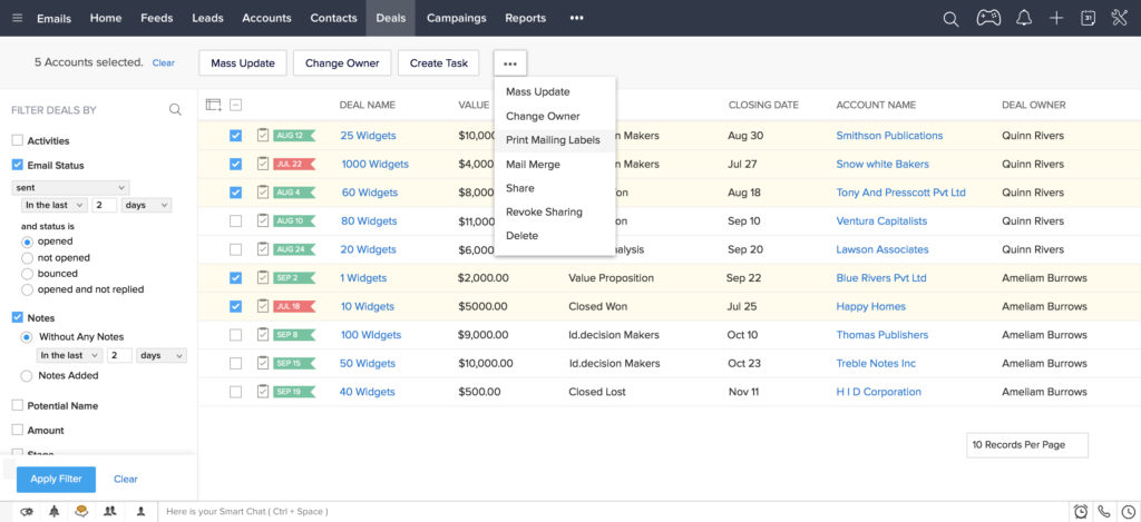
2. Sales Pipeline Management
A robust sales pipeline is essential for tracking leads, managing opportunities, and closing deals. The demo should showcase the CRM’s sales pipeline features, including lead scoring, deal stages, and sales forecasting. Can you easily visualize your sales pipeline? Can you track the progress of each deal and identify potential bottlenecks? A well-designed sales pipeline will empower your sales team to work more efficiently.
3. Marketing Automation Capabilities
Marketing automation can save you time and improve the effectiveness of your marketing campaigns. The demo should highlight the CRM’s marketing automation features, such as email marketing, lead nurturing, and social media integration. Can you automate repetitive tasks, such as sending follow-up emails or segmenting your audience? Automation can free up your marketing team to focus on more strategic initiatives.
4. Reporting and Analytics
Data is the lifeblood of any business. The demo should provide a clear overview of the CRM’s reporting and analytics capabilities. Can you generate custom reports to track key metrics? Can you visualize your data with charts and graphs? A good reporting system will give you the insights you need to make data-driven decisions.
5. Mobile Accessibility
In today’s fast-paced world, mobile accessibility is a must-have. The demo should demonstrate the CRM’s mobile app or mobile-friendly interface. Can you access your data on the go? Can you update records and track activities from your smartphone or tablet? Mobile accessibility will empower your team to stay connected and productive, wherever they are.
6. Integration with Other Tools
As mentioned earlier, integration is key. During the demo, ask about the CRM’s integration capabilities. Does it integrate with your existing tools, such as email marketing platforms, accounting software, and social media channels? Seamless integration will streamline your workflow and avoid data silos.
7. Pricing and Support
Don’t forget to inquire about pricing and support. Ask about the different pricing plans and what features are included in each plan. Also, ask about the vendor’s customer support and training resources. Do they offer phone support, email support, or live chat? Do they provide online tutorials and knowledge bases? A good vendor will offer comprehensive support to help you get the most out of their system.
Key Features to Expect in a Small Business CRM Demo
Now, let’s dive into some specific features you should expect to see showcased in a small business CRM demo:
Contact Management
This is the foundation of any CRM. The demo should demonstrate how the system allows you to store and manage contact information, including names, addresses, phone numbers, email addresses, and social media profiles. Look for features like:
- Contact segmentation: Grouping contacts based on criteria like industry, location, or purchase history.
- Contact tagging: Adding tags to contacts for easy filtering and organization.
- Contact enrichment: Automatically adding contact details from public sources.
Lead Management
A CRM should help you capture, qualify, and nurture leads. The demo should showcase how the system helps you track leads through the sales pipeline. Look for features like:
- Lead capture forms: Creating forms to capture leads from your website or landing pages.
- Lead scoring: Assigning scores to leads based on their behavior and demographics.
- Lead assignment: Automatically assigning leads to sales representatives.
- Lead nurturing: Sending automated email sequences to nurture leads.
Sales Pipeline Management
This is where the magic happens. The demo should demonstrate how the system helps you visualize and manage your sales pipeline. Look for features like:
- Deal stages: Defining the stages of your sales process (e.g., prospecting, qualification, proposal, negotiation, closed won).
- Deal tracking: Tracking the progress of each deal through the pipeline.
- Sales forecasting: Predicting future sales based on your pipeline data.
- Activity tracking: Logging calls, emails, and meetings related to each deal.
Marketing Automation
Automate your marketing efforts to save time and improve efficiency. The demo should showcase features like:
- Email marketing: Sending targeted email campaigns to your contacts.
- Workflow automation: Automating tasks such as sending follow-up emails or updating contact information.
- Landing page creation: Creating landing pages to capture leads.
- Social media integration: Connecting your CRM to your social media accounts.
Reporting and Analytics
Gain insights into your sales performance and customer behavior. The demo should demonstrate how the system helps you track key metrics. Look for features like:
- Custom reports: Creating reports to track specific data points.
- Dashboards: Visualizing your data with charts and graphs.
- Sales performance reports: Tracking sales revenue, deal closure rates, and other key metrics.
- Customer behavior reports: Analyzing customer interactions and preferences.
Integration with Other Tools
Ensure seamless integration with your existing tools. The demo should showcase how the system integrates with:
- Email marketing platforms: Such as Mailchimp, Constant Contact, or Campaign Monitor.
- Accounting software: Such as QuickBooks or Xero.
- Social media channels: Such as Facebook, Twitter, and LinkedIn.
- Other business applications: Such as project management software or e-commerce platforms.
Preparing for Your Small Business CRM Demo
To make the most of your CRM demo, it’s important to prepare beforehand. Here’s a checklist to help you get ready:
1. Define Your Needs
Before the demo, take some time to define your specific needs. What are your business goals? What are your pain points? What are the key features you’re looking for in a CRM? Having a clear understanding of your needs will help you evaluate the system and determine if it’s the right fit.
2. Research Potential Vendors
Do your research and identify potential CRM vendors. Read reviews, compare features, and check pricing. This will help you narrow down your options and choose the vendors you want to see a demo from.
3. Prepare a List of Questions
Create a list of questions to ask during the demo. This will ensure you get all the information you need to make an informed decision. Focus on the features and functionality that are most important to your business.
4. Gather Your Data
If possible, gather some sample data to use during the demo. This will allow you to see how the system handles your specific data and how it can be customized to fit your needs.
5. Involve Key Stakeholders
If you have a team, involve key stakeholders in the demo process. This will ensure that everyone is on board and that the system meets the needs of your entire team.
6. Take Notes
Take detailed notes during the demo. This will help you remember the key features and functionality of the system and compare it to other options.
7. Ask for a Trial Period
If possible, ask for a trial period after the demo. This will allow you to test the system with your own data and see how it works in practice.
Making the Right Choice: Selecting the Best Small Business CRM
Choosing the right CRM is a significant decision, but it doesn’t have to be overwhelming. By following the steps outlined in this article, you can confidently evaluate different CRM systems and select the one that best fits your business needs. Here’s a recap of the key considerations:
1. Assess Your Needs
Clearly define your business goals and pain points. Identify the features and functionality that are most important to you.
2. Research Potential Vendors
Read reviews, compare features, and check pricing. Narrow down your options to a few potential vendors.
3. Schedule Demos
Schedule demos with your top choices. Prepare a list of questions to ask during the demo.
4. Evaluate the Demos
Assess the user interface, explore key features, evaluate integration capabilities, and assess customer support. Take detailed notes.
5. Consider Customization and Scalability
Ensure the system can be customized to fit your specific needs and that it can scale as your business grows.
6. Compare Pricing and Support
Compare the different pricing plans and evaluate the vendor’s customer support and training resources.
7. Ask for a Trial Period
If possible, ask for a trial period to test the system with your own data.
8. Make a Decision
Based on your evaluation, make a decision and choose the CRM that best fits your needs.
Conclusion: Embrace the Power of a Small Business CRM
A small business CRM is more than just a software tool; it’s a strategic investment in your business’s future. By streamlining your processes, improving customer relationships, and gaining valuable insights, a CRM can help you achieve your business goals and thrive in today’s competitive market. Don’t underestimate the power of a well-chosen CRM to revolutionize your operations and drive sustainable growth.
Take the first step towards transforming your business today. Schedule a small business CRM demo and experience the difference!


